Easy way to Learn Pivot Table Step By Step - Tutorial - Case Study 3

Using Microsoft Excel 2007

Case3:

Here, create an excel as below:

We are trying to find the total score by each student

Highlight A1 till C3. Click Insert -> Pivot Table -> Pivot Table

Click Ok.

Drag the Student column inside row label as below

We would like to see the marks and total as sub items for each student.

Drag the English and Maths column inside Values as below. This will automatically put the grand total (sigma sign) inside Column Labels as below

Now, just drag the (sigma values) from column labels to Row Labels. So that, the labels shows under each name as sub items as below

Now, rename the sum of English to English (as it is not sum actually) and also Sum of maths to Maths as below

Click Sum of English -> Value Field Settings.

Change the Custom Name from “Sum of English” to “English_Mark” as below (note: we can’t set English here, as it is already a valid column name)

Click OK

Similarly, do it for Sum of Maths. It will show finally as,

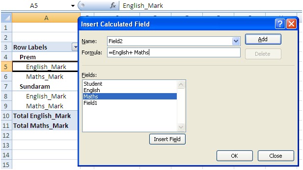
Now, total is a new field, which we need to create.

Under Options -> Formulas -> Click Calculated fields. As below

It will show below screen

Highlight English. Click Insert Field.

Then, type a + sign and highlight Maths. Click Insert Field as below

Click ok.

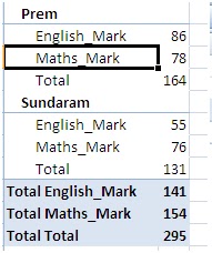
You will see the desired result:

Rename the Sum of Field2 to “Total” (the same way, done earlier for English_Mark). Below is the final expected screen.

Under Options -> unhighlight “Field Headers”

Resultant screen will look like:

  Done

Continue Case Study: http://learneasyhere.blogspot.in/2012/12/easy-way-to-learn-pivot-table-step-by_972.html