Easy way to Learn Pivot Table Step By Step - Tutorial - Case Study 2

Using Microsoft Excel 2007

Case2:

Create an excel as below

We don’t want to change the look, but we would like add filters via pivot table (not by using Data -> Filter, because in excel 2003 or before, this filtering would not allow multi select)

Highlight the cells from A1 to G5. Click Insert -> Pivot Table -> Pivot Table.

It opens a blank pivot table in a new worksheet as below. Drag the selected columns as below into Row Labels, so that, it gets displayed as below

Here, we see that, all the rows are stacked inside each other. We want all the rows displayed in the normal look. To do this,

Click Onsite column in Row Labels -> Field Settings as below

In the below screen, select the “Show items labels in tabular form”. Click Ok. 

You won't  see any change in the appearance, because, this is the last field as below

Now, do the same for Designation.

Click Designation -> Field Settings -> Under Layout & Print -> check “Show item labels in tabular form”. Click ok. You will get the below screen, where “Onsite” column shows and its values are displayed in rows.

Now, do the same for Emp Name.

Click Emp Name -> Field Settings -> Under Layout & Print -> check “Show item labels in tabular form”. Click ok. You will get the below screen, where “Designation” column shows and its values are displayed in rows.

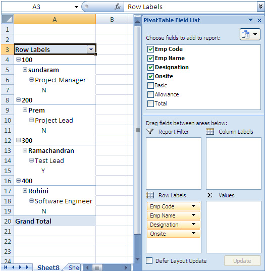
Now, do the same for Emp Code.

Click Emp Code -> Field Settings -> Under Layout & Print -> check “Show item labels in tabular form”. Click ok. You will get the below screen, where “Emp Name” column shows and its values are displayed in rows.

Now, we see that, Sum Total is displaying for each value, which looks odd. We can remove this.

Click Emp Code -> Field Settings -> select None. Check “Include new items in manual filter”  

Click OK.

You will see below screen

Similarly, do the above step for other 3 columns (Emp Name, Designation, Onsite). You will get the screen as below

This pivot table is not in classic look (they way it works in excel 2003). This will enable us, not only to filter Emp Code, but also other columns as well. TO do this,

Right Click Row Labels -> PivotTable Options… as below

Under Display Tab -> check “Classic Pivot Table layout…” as below.

Click OK.

Now, you can see filters in all fields and look changes to classic as well (as shown below)

Now, Drag Basic, Allowance and Total inside the Values box as below, You will get the screen as below:

  Done.

Continue Case Study: http://learneasyhere.blogspot.in/2012/12/easy-way-to-learn-pivot-table-step-by_8667.html