Easy way to Learn Pivot Table Step By Step - Tutorial - Case Study 6

Using Microsoft Excel 2007

Case6:

Create an excel with below data :

Now, highlight A1 till D10.

Click Insert  -> Pivot Table -> Pivot Table

Click ok.

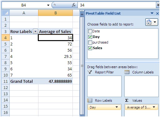
In the new worksheet, drag the  Day inside Row Labels.

Drag the sales inside Values as below

To change the Sum of Sales to Average of Sales -> Click the small down arrow near Sum of Sales -> Click “Value Field Settings”

Select “Average” as below

Click OK.

Now, the data shows on an average,  on Monday, Tuesday, wed, fri, sat, sun, what is the sales average as below:

Now, we want to highlight any sales less < 50 in red and above 49 is green.

To do this,

Highlight B4 cell.

Select Conditional formatting -> Manage rules as below:

It will display below screen

Click new Rule.. button

In the below screen,

Select “All cells showing “Average of Sales” values

Highlight “Format only cells that contain”

Enter the range from 0 to 49 as below:

Click Format button in the above screen,

Select “light red” color as below

Click Ok.

Click ok.

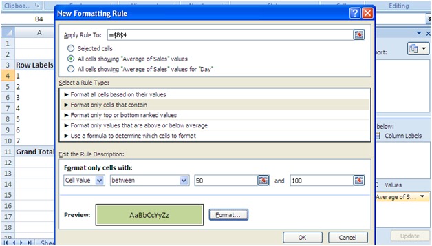
Click New Rule.. button again.

In the below screen,

Select “All cells showing “Average of Sales” values

Highlight “Format only cells that contain”

Enter the range from 50 to 100 as below:

Click format -> select “light green” color. Click Ok.

Click Ok.

Click Ok.

You will see color coding as below:

Done

Continue Case Study:

Easy way to Learn Pivot Table Step By Step - Tutorial - Case Study 5

Using Microsoft Excel 2007

 

Case5:

Create an excel with below data :

We are trying to find the average weight of people at each age.

Highlight from A1 to C5.

Click Insert -> Pivot Table -> Pivot table

Click Ok

First, Drag the Age column inside Row Label box as below

Now, Drag the Name inside Row Labels box as below

Click down arrow in Age -> Click Field Settings

In layout & Print Tab -> Check “Show item labels in tabular form” as below

Click Ok

You will see below screen

Now, Drag the Weight inside Values as below

Since we need to know average weight at each age, Sum of weight is not correct.

To do this, Click Downarrow in Sum of Weight -> Click Value Field Settings -> Select Average -> Click ok

You will get the desired result as below:

It shows 25 Total, which looks meaning less. To change this,

Click Downarrow in Age Under Row Labels -> Click Field Settings -> Select Custom -> Highlight “Average” as below

Click Ok

You will get  below screen

To change Row Labels, you can just rename as below

Click the – sign and you can see average of weight as below:

Done


Continue Case Study: http://learneasyhere.blogspot.in/2012/12/easy-way-to-learn-pivot-table-step-by_6055.html

Easy way to Learn Pivot Table Step By Step - Tutorial - Case Study 4

Using Microsoft Excel 2007

 

Case4:

Create an excel with below data :

Let’s say, we need to pull the report (month wise turnover), even though here, we have details on each day wise report.

TO do this,

Highlight the A1 till C5.

Click Insert -> pivot Table -> pivot table. Click ok.

In the new sheet,

Drag the “purchased on” inside the Row labels box as below:

Here, we see that, it is showing day wise report. To change this,

Click the down arrow in “purchased on” under Row labels -> click Field Settings.

Click Number format button in the below screen

Under Category: Make sure Date is highlighted.

Under Type: highlight “Mar-01” as below

Click ok

Click OK

You will get the below screen (monthwise)

Now, drag the Product inside Row Labels as below

Since we don’t need to see Product as subitem of Purchase on, we will change the look to classic.

To do this,

Click the down arrow key in Purchase On (under row labels) -> Field Settings

Goto “Layout  & Print”. Check “Show item labels in tabular form”

Click OK. You will get the below screen

Now, Drag the Price column inside “Values” as below

From this, we can see that,

On Jan, turnover is 35 Rs

On Feb, turnover is 40 Rs

On Mar, turnover is 50+34 = 84 (to view this, just click the – sign near mar, you can view the turnover as 84 as shown below:

Done

Continue Case Study: http://learneasyhere.blogspot.in/2012/12/easy-way-to-learn-pivot-table-step-by_110.html

Easy way to Learn Pivot Table Step By Step - Tutorial - Case Study 3

Using Microsoft Excel 2007

Case3:

Here, create an excel as below:

We are trying to find the total score by each student

Highlight A1 till C3. Click Insert -> Pivot Table -> Pivot Table

Click Ok.

Drag the Student column inside row label as below

We would like to see the marks and total as sub items for each student.

Drag the English and Maths column inside Values as below. This will automatically put the grand total (sigma sign) inside Column Labels as below

Now, just drag the (sigma values) from column labels to Row Labels. So that, the labels shows under each name as sub items as below

Now, rename the sum of English to English (as it is not sum actually) and also Sum of maths to Maths as below

Click Sum of English -> Value Field Settings.

Change the Custom Name from “Sum of English” to “English_Mark” as below (note: we can’t set English here, as it is already a valid column name)

Click OK

Similarly, do it for Sum of Maths. It will show finally as,

Now, total is a new field, which we need to create.

Under Options -> Formulas -> Click Calculated fields. As below

It will show below screen

Highlight English. Click Insert Field.

Then, type a + sign and highlight Maths. Click Insert Field as below

Click ok.

You will see the desired result:

Rename the Sum of Field2 to “Total” (the same way, done earlier for English_Mark). Below is the final expected screen.

Under Options -> unhighlight “Field Headers”

Resultant screen will look like:

  Done

Continue Case Study: http://learneasyhere.blogspot.in/2012/12/easy-way-to-learn-pivot-table-step-by_972.html