This is to understand how list can be added and how macros
can be written
Open the Excel, Rename Sheet1 as List and enter the name as
below

Click Formulas -> Define Name
Give the name as “NameList” and select the Range from A2
till A15 in List Sheet. It will show the below screen

Click OK
Now, Open Sheet2 and enter the data as shown below:

Now, highlight B2 to B4. Click Data -> Data Validation -> Data
Validation as below:

It will display the below screen. Select List from Dropdown.
Type =Namelist as below

Click OK
From now, you will be able to select the Names as dropdown
box in B2, B3, B4 cell as below

Now, we will learn how to add a checkbox.
Click the More Command from the below link:

You will see the below screen:

Change the Popular Commands from Dropdown to Developer tab
as below

Select Control. Click Add as below

Click OK
In below, you can see the control button showing in Quick
Access Toolbar as below

Now. Click the Insert -> Select the Checkbox control
under form control as below

Click over D1 cell as below, it will place the checkbox
control. Adjust the cell such that, checkbox control looks like, it get placed
inside the cell D1 as below

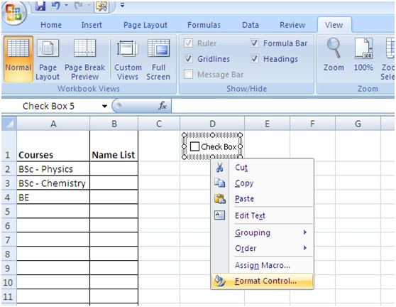
Right Click the checkbox control -> Click “Format
control” as below

Under Web tab, change the Name displayed as below

Click OK.
Now, Right Click the control once again as below. Click Edit
Text
Click Edit Text
Change the Name to “Multi Select” as below

Now, goto Sheet “List”. Highlight Cell D1, and Change the
Name of this Cell from B1 to EditMode as below

Now, Goto Sheet2, Right Click the checkbox control as below

Click Format Control.
In Control Tab, give the link Name as “EditMode” as below

Click OK
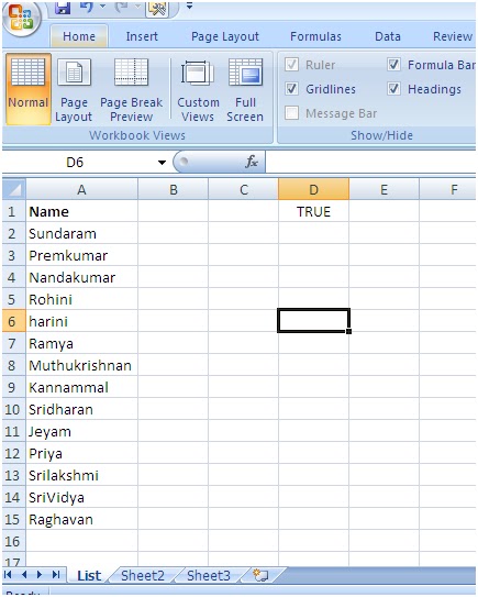
The above steps, ensures, that, based on the value selected
in the checkbox, Cell D1 in Sheet “List” will change to False/True.
Let’s check the box in Sheet2 as below

Goto Sheet “List”. You can see, Cell D1 shows True as below
Now, right click Sheet2 -> View Code as below

It will open VBA screen.
Write the below code
Option Explicit
Private Sub Worksheet_Change(ByVal Target As Range)
Dim rngDV As Range
Dim oldVal As String
Dim newVal As String
Dim strSep As String
Dim rngEdit As Range
Set rngEdit =
Worksheets("List").Range("EditMode")
strSep = Chr(10) 'line break separator
If Target.Count > 1 Then GoTo exitHandler
On Error Resume Next
Set rngDV = Cells.SpecialCells(xlCellTypeAllValidation)
On Error GoTo exitHandler
If rngDV Is Nothing Then GoTo exitHandler
If rngEdit.Value = True Then
If
Intersect(Target, rngDV) Is Nothing Then
'do nothing
Else
Application.EnableEvents = False
newVal =
Target.Value
Application.Undo
oldVal =
Target.Value
Target.Value =
newVal
If Target.Column
= 2 Or Target.Column = 4 Then
If oldVal =
"" Then
'do nothing
Else
If newVal =
"" Then
'do nothing
Else
Target.Value
= oldVal _
&
strSep & newVal
End If
End If
End If
End If
End If
exitHandler:
Application.EnableEvents = True
End Sub

Close the VBA window
Ensure, the Control
is not design mode by ensuring Design mode is not highlighted, by
verifying the below screen

It should look like

Save this. Give filename as “List_Macros”.
Close the Excel.
Reopen the File “List_Macros.xlsx”
With Checkbox unchecked, select some names as below

Now, put checkmark in the multi select. Now Add “Rohini” in
addition to the existing name “SriVidya”
If it didn’t add, macros is not working.
Right Click Sheet 2 -> View Code.
If the code is not there, reenter the code once again as
given above.
Click Save. You might get the below screen

Click No.
In the below screen, ensure that, you select the file type
as below and click Save

Click Save.
Now, close the VBA Screen. Close the Excel.
Reopen the Excel.
If the macros are disabled, you can enable by clicking the
Options and selecting the below option.

Click OK
Now, check the multi select box as below

Now select 2 names for Bsc Physics as below. It will allow
you to multi display as below

Done


